45. Packet Framework
45.1. Design Objectives
The main design objectives for the DPDK Packet Framework are:
- Provide standard methodology to build complex packet processing pipelines. Provide reusable and extensible templates for the commonly used pipeline functional blocks;
- Provide capability to switch between pure software and hardware-accelerated implementations for the same pipeline functional block;
- Provide the best trade-off between flexibility and performance. Hardcoded pipelines usually provide the best performance, but are not flexible, while developing flexible frameworks is never a problem, but performance is usually low;
- Provide a framework that is logically similar to Open Flow.
45.2. Overview
Packet processing applications are frequently structured as pipelines of multiple stages, with the logic of each stage glued around a lookup table. For each incoming packet, the table defines the set of actions to be applied to the packet, as well as the next stage to send the packet to.
The DPDK Packet Framework minimizes the development effort required to build packet processing pipelines by defining a standard methodology for pipeline development, as well as providing libraries of reusable templates for the commonly used pipeline blocks.
The pipeline is constructed by connecting the set of input ports with the set of output ports through the set of tables in a tree-like topology. As result of lookup operation for the current packet in the current table, one of the table entries (on lookup hit) or the default table entry (on lookup miss) provides the set of actions to be applied on the current packet, as well as the next hop for the packet, which can be either another table, an output port or packet drop.
An example of packet processing pipeline is presented in Fig. 45.1:
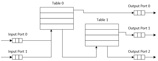
Fig. 45.1 Example of Packet Processing Pipeline where Input Ports 0 and 1 are Connected with Output Ports 0, 1 and 2 through Tables 0 and 1
45.3. Port Library Design
45.3.1. Port Types
Table 45.1 is a non-exhaustive list of ports that can be implemented with the Packet Framework.
| # | Port type | Description |
|---|---|---|
| 1 | SW ring | SW circular buffer used for message passing between the application threads. Uses the DPDK rte_ring primitive. Expected to be the most commonly used type of port. |
| 2 | HW ring | Queue of buffer descriptors used to interact with NIC, switch or accelerator ports. For NIC ports, it uses the DPDK rte_eth_rx_queue or rte_eth_tx_queue primitives. |
| 3 | IP reassembly | Input packets are either IP fragments or complete IP datagrams. Output packets are complete IP datagrams. |
| 4 | IP fragmentation | Input packets are jumbo (IP datagrams with length bigger than MTU) or non-jumbo packets. Output packets are non-jumbo packets. |
| 5 | Traffic manager | Traffic manager attached to a specific NIC output port, performing congestion management and hierarchical scheduling according to pre-defined SLAs. |
| 6 | KNI | Send/receive packets to/from Linux kernel space. |
| 7 | Source | Input port used as packet generator. Similar to Linux kernel /dev/zero character device. |
| 8 | Sink | Output port used to drop all input packets. Similar to Linux kernel /dev/null character device. |
| 9 | Sym_crypto | Output port used to extract DPDK Cryptodev operations from a fixed offset of the packet and then enqueue to the Cryptodev PMD. Input port used to dequeue the Cryptodev operations from the Cryptodev PMD and then retrieve the packets from them. |
45.3.2. Port Interface
Each port is unidirectional, i.e. either input port or output port. Each input/output port is required to implement an abstract interface that defines the initialization and run-time operation of the port. The port abstract interface is described in.
| # | Port Operation | Description |
|---|---|---|
| 1 | Create | Create the low-level port object (e.g. queue). Can internally allocate memory. |
| 2 | Free | Free the resources (e.g. memory) used by the low-level port object. |
| 3 | RX | Read a burst of input packets. Non-blocking operation. Only defined for input ports. |
| 4 | TX | Write a burst of input packets. Non-blocking operation. Only defined for output ports. |
| 5 | Flush | Flush the output buffer. Only defined for output ports. |
45.4. Table Library Design
45.4.1. Table Types
Table 45.3 is a non-exhaustive list of types of tables that can be implemented with the Packet Framework.
| # | Table Type | Description |
|---|---|---|
| 1 | Hash table | Lookup key is n-tuple based. Typically, the lookup key is hashed to produce a signature that is used to identify a bucket of entries where the lookup key is searched next. The signature associated with the lookup key of each input packet is either read from the packet descriptor (pre-computed signature) or computed at table lookup time. The table lookup, add entry and delete entry operations, as well as any other pipeline block that pre-computes the signature all have to use the same hashing algorithm to generate the signature. Typically used to implement flow classification tables, ARP caches, routing table for tunnelling protocols, etc. |
| 2 | Longest Prefix Match (LPM) | Lookup key is the IP address. Each table entries has an associated IP prefix (IP and depth). The table lookup operation selects the IP prefix that is matched by the lookup key; in case of multiple matches, the entry with the longest prefix depth wins. Typically used to implement IP routing tables. |
| 3 | Access Control List (ACLs) | Lookup key is 7-tuple of two VLAN/MPLS labels, IP destination address, IP source addresses, L4 protocol, L4 destination port, L4 source port. Each table entry has an associated ACL and priority. The ACL contains bit masks for the VLAN/MPLS labels, IP prefix for IP destination address, IP prefix for IP source addresses, L4 protocol and bitmask, L4 destination port and bit mask, L4 source port and bit mask. The table lookup operation selects the ACL that is matched by the lookup key; in case of multiple matches, the entry with the highest priority wins. Typically used to implement rule databases for firewalls, etc. |
| 4 | Pattern matching search | Lookup key is the packet payload. Table is a database of patterns, with each pattern having a priority assigned. The table lookup operation selects the patterns that is matched by the input packet; in case of multiple matches, the matching pattern with the highest priority wins. |
| 5 | Array | Lookup key is the table entry index itself. |
45.4.2. Table Interface
Each table is required to implement an abstract interface that defines the initialization and run-time operation of the table. The table abstract interface is described in Table 45.4.
| # | Table operation | Description |
|---|---|---|
| 1 | Create | Create the low-level data structures of the lookup table. Can internally allocate memory. |
| 2 | Free | Free up all the resources used by the lookup table. |
| 3 | Add entry | Add new entry to the lookup table. |
| 4 | Delete entry | Delete specific entry from the lookup table. |
| 5 | Lookup | Look up a burst of input packets and return a bit mask specifying the result of the lookup operation for each packet: a set bit signifies lookup hit for the corresponding packet, while a cleared bit a lookup miss. For each lookup hit packet, the lookup operation also returns a pointer to the table entry that was hit, which contains the actions to be applied on the packet and any associated metadata. For each lookup miss packet, the actions to be applied on the packet and any associated metadata are specified by the default table entry preconfigured for lookup miss. |
45.4.3. Hash Table Design
45.4.3.1. Hash Table Overview
Hash tables are important because the key lookup operation is optimized for speed: instead of having to linearly search the lookup key through all the keys in the table, the search is limited to only the keys stored in a single table bucket.
Associative Arrays
An associative array is a function that can be specified as a set of (key, value) pairs, with each key from the possible set of input keys present at most once. For a given associative array, the possible operations are:
- add (key, value): When no value is currently associated with key, then the (key, value ) association is created. When key is already associated value value0, then the association (key, value0) is removed and association (key, value) is created;
- delete key: When no value is currently associated with key, this operation has no effect. When key is already associated value, then association (key, value) is removed;
- lookup key: When no value is currently associated with key, then this operation returns void value (lookup miss). When key is associated with value, then this operation returns value. The (key, value) association is not changed.
The matching criterion used to compare the input key against the keys in the associative array is exact match, as the key size (number of bytes) and the key value (array of bytes) have to match exactly for the two keys under comparison.
Hash Function
A hash function deterministically maps data of variable length (key) to data of fixed size (hash value or key signature). Typically, the size of the key is bigger than the size of the key signature. The hash function basically compresses a long key into a short signature. Several keys can share the same signature (collisions).
High quality hash functions have uniform distribution. For large number of keys, when dividing the space of signature values into a fixed number of equal intervals (buckets), it is desirable to have the key signatures evenly distributed across these intervals (uniform distribution), as opposed to most of the signatures going into only a few of the intervals and the rest of the intervals being largely unused (non-uniform distribution).
Hash Table
A hash table is an associative array that uses a hash function for its operation. The reason for using a hash function is to optimize the performance of the lookup operation by minimizing the number of table keys that have to be compared against the input key.
Instead of storing the (key, value) pairs in a single list, the hash table maintains multiple lists (buckets). For any given key, there is a single bucket where that key might exist, and this bucket is uniquely identified based on the key signature. Once the key signature is computed and the hash table bucket identified, the key is either located in this bucket or it is not present in the hash table at all, so the key search can be narrowed down from the full set of keys currently in the table to just the set of keys currently in the identified table bucket.
The performance of the hash table lookup operation is greatly improved, provided that the table keys are evenly distributed among the hash table buckets, which can be achieved by using a hash function with uniform distribution. The rule to map a key to its bucket can simply be to use the key signature (modulo the number of table buckets) as the table bucket ID:
bucket_id = f_hash(key) % n_buckets;
By selecting the number of buckets to be a power of two, the modulo operator can be replaced by a bitwise AND logical operation:
bucket_id = f_hash(key) & (n_buckets - 1);
considering n_bits as the number of bits set in bucket_mask = n_buckets - 1, this means that all the keys that end up in the same hash table bucket have the lower n_bits of their signature identical. In order to reduce the number of keys in the same bucket (collisions), the number of hash table buckets needs to be increased.
In packet processing context, the sequence of operations involved in hash table operations is described in Fig. 45.2:
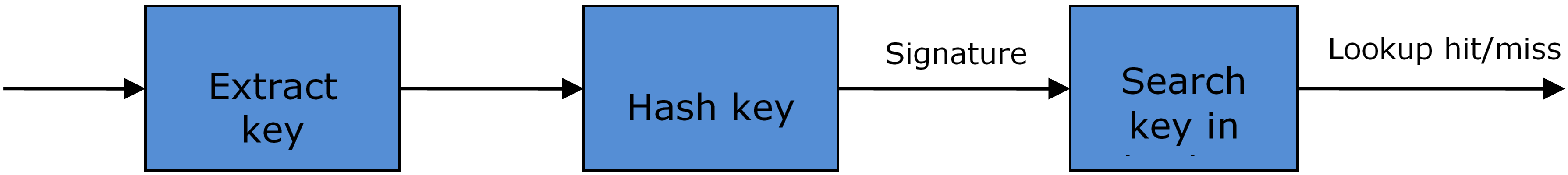
Fig. 45.2 Sequence of Steps for Hash Table Operations in a Packet Processing Context
45.4.3.2. Hash Table Use Cases
Flow Classification
Description: The flow classification is executed at least once for each input packet. This operation maps each incoming packet against one of the known traffic flows in the flow database that typically contains millions of flows.
Hash table name: Flow classification table
Number of keys: Millions
Key format: n-tuple of packet fields that uniquely identify a traffic flow/connection. Example: DiffServ 5-tuple of (Source IP address, Destination IP address, L4 protocol, L4 protocol source port, L4 protocol destination port). For IPv4 protocol and L4 protocols like TCP, UDP or SCTP, the size of the DiffServ 5-tuple is 13 bytes, while for IPv6 it is 37 bytes.
Key value (key data): actions and action meta-data describing what processing to be applied for the packets of the current flow. The size of the data associated with each traffic flow can vary from 8 bytes to kilobytes.
Address Resolution Protocol (ARP)
Description: Once a route has been identified for an IP packet (so the output interface and the IP address of the next hop station are known), the MAC address of the next hop station is needed in order to send this packet onto the next leg of the journey towards its destination (as identified by its destination IP address). The MAC address of the next hop station becomes the destination MAC address of the outgoing Ethernet frame.
Hash table name: ARP table
Number of keys: Thousands
Key format: The pair of (Output interface, Next Hop IP address), which is typically 5 bytes for IPv4 and 17 bytes for IPv6.
Key value (key data): MAC address of the next hop station (6 bytes).
45.4.3.3. Hash Table Types
Table 45.5 lists the hash table configuration parameters shared by all different hash table types.
| # | Parameter | Details |
|---|---|---|
| 1 | Key size | Measured as number of bytes. All keys have the same size. |
| 2 | Key value (key data) size | Measured as number of bytes. |
| 3 | Number of buckets | Needs to be a power of two. |
| 4 | Maximum number of keys | Needs to be a power of two. |
| 5 | Hash function | Examples: jhash, CRC hash, etc. |
| 6 | Hash function seed | Parameter to be passed to the hash function. |
| 7 | Key offset | Offset of the lookup key byte array within the packet meta-data stored in the packet buffer. |
45.4.3.3.1. Bucket Full Problem
On initialization, each hash table bucket is allocated space for exactly 4 keys. As keys are added to the table, it can happen that a given bucket already has 4 keys when a new key has to be added to this bucket. The possible options are:
- Least Recently Used (LRU) Hash Table. One of the existing keys in the bucket is deleted and the new key is added in its place. The number of keys in each bucket never grows bigger than 4. The logic to pick the key to be dropped from the bucket is LRU. The hash table lookup operation maintains the order in which the keys in the same bucket are hit, so every time a key is hit, it becomes the new Most Recently Used (MRU) key, i.e. the last candidate for drop. When a key is added to the bucket, it also becomes the new MRU key. When a key needs to be picked and dropped, the first candidate for drop, i.e. the current LRU key, is always picked. The LRU logic requires maintaining specific data structures per each bucket.
- Extendable Bucket Hash Table. The bucket is extended with space for 4 more keys. This is done by allocating additional memory at table initialization time, which is used to create a pool of free keys (the size of this pool is configurable and always a multiple of 4). On key add operation, the allocation of a group of 4 keys only happens successfully within the limit of free keys, otherwise the key add operation fails. On key delete operation, a group of 4 keys is freed back to the pool of free keys when the key to be deleted is the only key that was used within its group of 4 keys at that time. On key lookup operation, if the current bucket is in extended state and a match is not found in the first group of 4 keys, the search continues beyond the first group of 4 keys, potentially until all keys in this bucket are examined. The extendable bucket logic requires maintaining specific data structures per table and per each bucket.
| # | Parameter | Details |
|---|---|---|
| 1 | Number of additional keys | Needs to be a power of two, at least equal to 4. |
45.4.3.3.2. Signature Computation
The possible options for key signature computation are:
- Pre-computed key signature. The key lookup operation is split between two CPU cores. The first CPU core (typically the CPU core that performs packet RX) extracts the key from the input packet, computes the key signature and saves both the key and the key signature in the packet buffer as packet meta-data. The second CPU core reads both the key and the key signature from the packet meta-data and performs the bucket search step of the key lookup operation.
- Key signature computed on lookup (“do-sig” version). The same CPU core reads the key from the packet meta-data, uses it to compute the key signature and also performs the bucket search step of the key lookup operation.
| # | Parameter | Details |
|---|---|---|
| 1 | Signature offset | Offset of the pre-computed key signature within the packet meta-data. |
45.4.3.3.3. Key Size Optimized Hash Tables
For specific key sizes, the data structures and algorithm of key lookup operation can be specially handcrafted for further performance improvements, so following options are possible:
- Implementation supporting configurable key size.
- Implementation supporting a single key size. Typical key sizes are 8 bytes and 16 bytes.
45.4.3.4. Bucket Search Logic for Configurable Key Size Hash Tables
The performance of the bucket search logic is one of the main factors influencing the performance of the key lookup operation. The data structures and algorithm are designed to make the best use of Intel CPU architecture resources like: cache memory space, cache memory bandwidth, external memory bandwidth, multiple execution units working in parallel, out of order instruction execution, special CPU instructions, etc.
The bucket search logic handles multiple input packets in parallel. It is built as a pipeline of several stages (3 or 4), with each pipeline stage handling two different packets from the burst of input packets. On each pipeline iteration, the packets are pushed to the next pipeline stage: for the 4-stage pipeline, two packets (that just completed stage 3) exit the pipeline, two packets (that just completed stage 2) are now executing stage 3, two packets (that just completed stage 1) are now executing stage 2, two packets (that just completed stage 0) are now executing stage 1 and two packets (next two packets to read from the burst of input packets) are entering the pipeline to execute stage 0. The pipeline iterations continue until all packets from the burst of input packets execute the last stage of the pipeline.
The bucket search logic is broken into pipeline stages at the boundary of the next memory access. Each pipeline stage uses data structures that are stored (with high probability) into the L1 or L2 cache memory of the current CPU core and breaks just before the next memory access required by the algorithm. The current pipeline stage finalizes by prefetching the data structures required by the next pipeline stage, so given enough time for the prefetch to complete, when the next pipeline stage eventually gets executed for the same packets, it will read the data structures it needs from L1 or L2 cache memory and thus avoid the significant penalty incurred by L2 or L3 cache memory miss.
By prefetching the data structures required by the next pipeline stage in advance (before they are used) and switching to executing another pipeline stage for different packets, the number of L2 or L3 cache memory misses is greatly reduced, hence one of the main reasons for improved performance. This is because the cost of L2/L3 cache memory miss on memory read accesses is high, as usually due to data dependency between instructions, the CPU execution units have to stall until the read operation is completed from L3 cache memory or external DRAM memory. By using prefetch instructions, the latency of memory read accesses is hidden, provided that it is preformed early enough before the respective data structure is actually used.
By splitting the processing into several stages that are executed on different packets (the packets from the input burst are interlaced), enough work is created to allow the prefetch instructions to complete successfully (before the prefetched data structures are actually accessed) and also the data dependency between instructions is loosened. For example, for the 4-stage pipeline, stage 0 is executed on packets 0 and 1 and then, before same packets 0 and 1 are used (i.e. before stage 1 is executed on packets 0 and 1), different packets are used: packets 2 and 3 (executing stage 1), packets 4 and 5 (executing stage 2) and packets 6 and 7 (executing stage 3). By executing useful work while the data structures are brought into the L1 or L2 cache memory, the latency of the read memory accesses is hidden. By increasing the gap between two consecutive accesses to the same data structure, the data dependency between instructions is loosened; this allows making the best use of the super-scalar and out-of-order execution CPU architecture, as the number of CPU core execution units that are active (rather than idle or stalled due to data dependency constraints between instructions) is maximized.
The bucket search logic is also implemented without using any branch instructions. This avoids the important cost associated with flushing the CPU core execution pipeline on every instance of branch misprediction.
45.4.3.4.1. Configurable Key Size Hash Table
Fig. 45.3, Table 45.8 and Table 45.9 detail the main data structures used to implement configurable key size hash tables (either LRU or extendable bucket, either with pre-computed signature or “do-sig”).
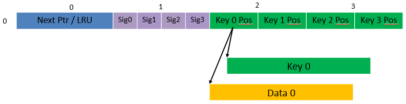
Fig. 45.3 Data Structures for Configurable Key Size Hash Tables
| # | Array name | Number of entries | Entry size (bytes) | Description |
|---|---|---|---|---|
| 1 | Bucket array | n_buckets (configurable) | 32 | Buckets of the hash table. |
| 2 | Bucket extensions array | n_buckets_ext (configurable) | 32 | This array is only created for extendable bucket tables. |
| 3 | Key array | n_keys | key_size (configurable) | Keys added to the hash table. |
| 4 | Data array | n_keys | entry_size (configurable) | Key values (key data) associated with the hash table keys. |
| # | Field name | Field size (bytes) | Description |
|---|---|---|---|
| 1 | Next Ptr/LRU | 8 | For LRU tables, this fields represents the LRU list for the current bucket stored as array of 4 entries of 2 bytes each. Entry 0 stores the index (0 .. 3) of the MRU key, while entry 3 stores the index of the LRU key. For extendable bucket tables, this field represents the next pointer (i.e. the pointer to the next group of 4 keys linked to the current bucket). The next pointer is not NULL if the bucket is currently extended or NULL otherwise. To help the branchless implementation, bit 0 (least significant bit) of this field is set to 1 if the next pointer is not NULL and to 0 otherwise. |
| 2 | Sig[0 .. 3] | 4 x 2 | If key X (X = 0 .. 3) is valid, then sig X bits 15 .. 1 store the most significant 15 bits of key X signature and sig X bit 0 is set to 1. If key X is not valid, then sig X is set to zero. |
| 3 | Key Pos [0 .. 3] | 4 x 4 | If key X is valid (X = 0 .. 3), then Key Pos X represents the index into the key array where key X is stored, as well as the index into the data array where the value associated with key X is stored. If key X is not valid, then the value of Key Pos X is undefined. |
Fig. 45.4 and Table 45.10 detail the bucket search pipeline stages (either LRU or extendable bucket, either with pre-computed signature or “do-sig”). For each pipeline stage, the described operations are applied to each of the two packets handled by that stage.
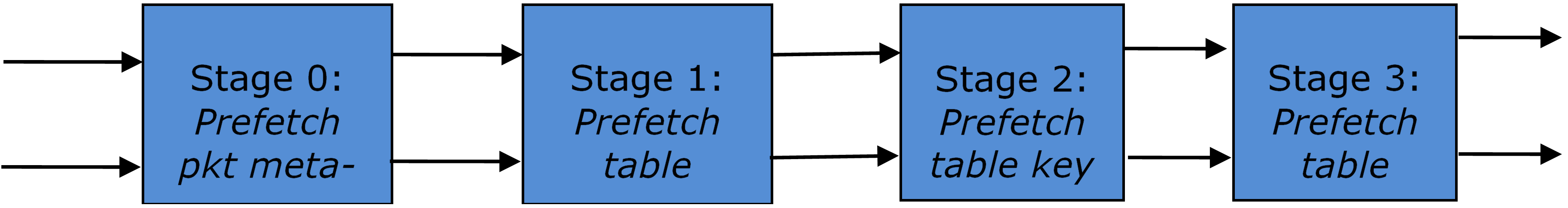
Fig. 45.4 Bucket Search Pipeline for Key Lookup Operation (Configurable Key Size Hash Tables)
| # | Stage name | Description |
|---|---|---|
| 0 | Prefetch packet meta-data | Select next two packets from the burst of input packets. Prefetch packet meta-data containing the key and key signature. |
| 1 | Prefetch table bucket | Read the key signature from the packet meta-data (for extendable bucket hash tables) or read the key from the packet meta-data and compute key signature (for LRU tables). Identify the bucket ID using the key signature. Set bit 0 of the signature to 1 (to match only signatures of valid keys from the table). Prefetch the bucket. |
| 2 | Prefetch table key | Read the key signatures from the bucket. Compare the signature of the input key against the 4 key signatures from the packet. As result, the following is obtained: match = equal to TRUE if there was at least one signature match and to FALSE in the case of no signature match; match_many = equal to TRUE is there were more than one signature matches (can be up to 4 signature matches in the worst case scenario) and to FALSE otherwise; match_pos = the index of the first key that produced signature match (only valid if match is true). For extendable bucket hash tables only, set match_many to TRUE if next pointer is valid. Prefetch the bucket key indicated by match_pos (even if match_pos does not point to valid key valid). |
| 3 | Prefetch table data | Read the bucket key indicated by match_pos. Compare the bucket key against the input key. As result, the following is obtained: match_key = equal to TRUE if the two keys match and to FALSE otherwise. Report input key as lookup hit only when both match and match_key are equal to TRUE and as lookup miss otherwise. For LRU tables only, use branchless logic to update the bucket LRU list (the current key becomes the new MRU) only on lookup hit. Prefetch the key value (key data) associated with the current key (to avoid branches, this is done on both lookup hit and miss). |
Additional notes:
- The pipelined version of the bucket search algorithm is executed only if there are at least 7 packets in the burst of input packets. If there are less than 7 packets in the burst of input packets, a non-optimized implementation of the bucket search algorithm is executed.
- Once the pipelined version of the bucket search algorithm has been executed for all the packets in the burst of input packets, the non-optimized implementation of the bucket search algorithm is also executed for any packets that did not produce a lookup hit, but have the match_many flag set. As result of executing the non-optimized version, some of these packets may produce a lookup hit or lookup miss. This does not impact the performance of the key lookup operation, as the probability of matching more than one signature in the same group of 4 keys or of having the bucket in extended state (for extendable bucket hash tables only) is relatively small.
Key Signature Comparison Logic
The key signature comparison logic is described in Table 45.11.
| # | mask | match (1 bit) | match_many (1 bit) | match_pos (2 bits) |
| 0 | 0000 | 0 | 0 | 00 |
| 1 | 0001 | 1 | 0 | 00 |
| 2 | 0010 | 1 | 0 | 01 |
| 3 | 0011 | 1 | 1 | 00 |
| 4 | 0100 | 1 | 0 | 10 |
| 5 | 0101 | 1 | 1 | 00 |
| 6 | 0110 | 1 | 1 | 01 |
| 7 | 0111 | 1 | 1 | 00 |
| 8 | 1000 | 1 | 0 | 11 |
| 9 | 1001 | 1 | 1 | 00 |
| 10 | 1010 | 1 | 1 | 01 |
| 11 | 1011 | 1 | 1 | 00 |
| 12 | 1100 | 1 | 1 | 10 |
| 13 | 1101 | 1 | 1 | 00 |
| 14 | 1110 | 1 | 1 | 01 |
| 15 | 1111 | 1 | 1 | 00 |
The input mask hash bit X (X = 0 .. 3) set to 1 if input signature is equal to bucket signature X and set to 0 otherwise. The outputs match, match_many and match_pos are 1 bit, 1 bit and 2 bits in size respectively and their meaning has been explained above.
As displayed in Table 45.12, the lookup tables for match and match_many can be collapsed into a single 32-bit value and the lookup table for match_pos can be collapsed into a 64-bit value. Given the input mask, the values for match, match_many and match_pos can be obtained by indexing their respective bit array to extract 1 bit, 1 bit and 2 bits respectively with branchless logic.
| Bit array | Hexadecimal value | |
| match | 1111_1111_1111_1110 | 0xFFFELLU |
| match_many | 1111_1110_1110_1000 | 0xFEE8LLU |
| match_pos | 0001_0010_0001_0011__0001_0010_0001_0000 | 0x12131210LLU |
The pseudo-code for match, match_many and match_pos is:
match = (0xFFFELLU >> mask) & 1;

match_many = (0xFEE8LLU >> mask) & 1;

match_pos = (0x12131210LLU >> (mask << 1)) & 3;
45.4.3.4.2. Single Key Size Hash Tables
Fig. 45.5, Fig. 45.6, Table 45.13 and Table 45.14 detail the main data structures used to implement 8-byte and 16-byte key hash tables (either LRU or extendable bucket, either with pre-computed signature or “do-sig”).
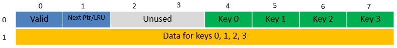
Fig. 45.5 Data Structures for 8-byte Key Hash Tables
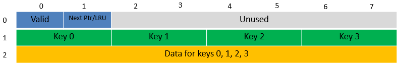
Fig. 45.6 Data Structures for 16-byte Key Hash Tables
| # | Array name | Number of entries | Entry size (bytes) | Description |
|---|---|---|---|---|
| 1 | Bucket array | n_buckets (configurable) | 8-byte key size: 64 + 4 x entry_size 16-byte key size: 128 + 4 x entry_size |
Buckets of the hash table. |
| 2 | Bucket extensions array | n_buckets_ext (configurable) | 8-byte key size: 64 + 4 x entry_size 16-byte key size: 128 + 4 x entry_size |
This array is only created for extendable bucket tables. |
| # | Field name | Field size (bytes) | Description |
|---|---|---|---|
| 1 | Valid | 8 | Bit X (X = 0 .. 3) is set to 1 if key X is valid or to 0 otherwise. Bit 4 is only used for extendable bucket tables to help with the implementation of the branchless logic. In this case, bit 4 is set to 1 if next pointer is valid (not NULL) or to 0 otherwise. |
| 2 | Next Ptr/LRU | 8 | For LRU tables, this fields represents the LRU list for the current bucket stored as array of 4 entries of 2 bytes each. Entry 0 stores the index (0 .. 3) of the MRU key, while entry 3 stores the index of the LRU key. For extendable bucket tables, this field represents the next pointer (i.e. the pointer to the next group of 4 keys linked to the current bucket). The next pointer is not NULL if the bucket is currently extended or NULL otherwise. |
| 3 | Key [0 .. 3] | 4 x key_size | Full keys. |
| 4 | Data [0 .. 3] | 4 x entry_size | Full key values (key data) associated with keys 0 .. 3. |
and detail the bucket search pipeline used to implement 8-byte and 16-byte key hash tables (either LRU or extendable bucket, either with pre-computed signature or “do-sig”). For each pipeline stage, the described operations are applied to each of the two packets handled by that stage.
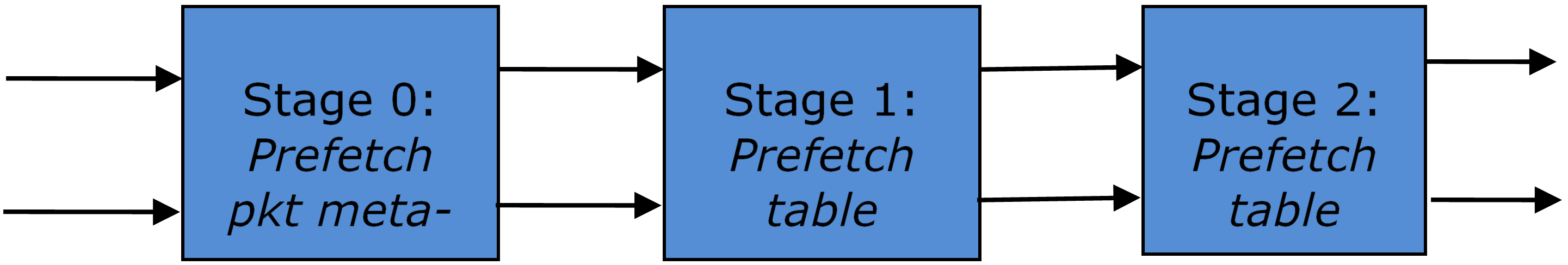
Fig. 45.7 Bucket Search Pipeline for Key Lookup Operation (Single Key Size Hash Tables)
| # | Stage name | Description |
|---|---|---|
| 0 | Prefetch packet meta-data |
|
| 1 | Prefetch table bucket |
|
| 2 | Prefetch table data |
|
Additional notes:
- The pipelined version of the bucket search algorithm is executed only if there are at least 5 packets in the burst of input packets. If there are less than 5 packets in the burst of input packets, a non-optimized implementation of the bucket search algorithm is executed.
- For extendable bucket hash tables only, once the pipelined version of the bucket search algorithm has been executed for all the packets in the burst of input packets, the non-optimized implementation of the bucket search algorithm is also executed for any packets that did not produce a lookup hit, but have the bucket in extended state. As result of executing the non-optimized version, some of these packets may produce a lookup hit or lookup miss. This does not impact the performance of the key lookup operation, as the probability of having the bucket in extended state is relatively small.
45.5. Pipeline Library Design
A pipeline is defined by:
- The set of input ports;
- The set of output ports;
- The set of tables;
- The set of actions.
The input ports are connected with the output ports through tree-like topologies of interconnected tables. The table entries contain the actions defining the operations to be executed on the input packets and the packet flow within the pipeline.
45.5.1. Connectivity of Ports and Tables
To avoid any dependencies on the order in which pipeline elements are created, the connectivity of pipeline elements is defined after all the pipeline input ports, output ports and tables have been created.
General connectivity rules:
- Each input port is connected to a single table. No input port should be left unconnected;
- The table connectivity to other tables or to output ports is regulated by the next hop actions of each table entry and the default table entry.
The table connectivity is fluid, as the table entries and the default table entry can be updated during run-time.
- A table can have multiple entries (including the default entry) connected to the same output port. A table can have different entries connected to different output ports. Different tables can have entries (including default table entry) connected to the same output port.
- A table can have multiple entries (including the default entry) connected to another table, in which case all these entries have to point to the same table. This constraint is enforced by the API and prevents tree-like topologies from being created (allowing table chaining only), with the purpose of simplifying the implementation of the pipeline run-time execution engine.
45.5.2. Port Actions
45.5.2.1. Port Action Handler
An action handler can be assigned to each input/output port to define actions to be executed on each input packet that is received by the port. Defining the action handler for a specific input/output port is optional (i.e. the action handler can be disabled).
For input ports, the action handler is executed after RX function. For output ports, the action handler is executed before the TX function.
The action handler can decide to drop packets.
45.5.3. Table Actions
45.5.3.1. Table Action Handler
An action handler to be executed on each input packet can be assigned to each table. Defining the action handler for a specific table is optional (i.e. the action handler can be disabled).
The action handler is executed after the table lookup operation is performed and the table entry associated with each input packet is identified. The action handler can only handle the user-defined actions, while the reserved actions (e.g. the next hop actions) are handled by the Packet Framework. The action handler can decide to drop the input packet.
45.5.3.2. Reserved Actions
The reserved actions are handled directly by the Packet Framework without the user being able to change their meaning through the table action handler configuration. A special category of the reserved actions is represented by the next hop actions, which regulate the packet flow between input ports, tables and output ports through the pipeline. Table 45.16 lists the next hop actions.
| # | Next hop action | Description |
|---|---|---|
| 1 | Drop | Drop the current packet. |
| 2 | Send to output port | Send the current packet to specified output port. The output port ID is metadata stored in the same table entry. |
| 3 | Send to table | Send the current packet to specified table. The table ID is metadata stored in the same table entry. |
45.5.3.3. User Actions
For each table, the meaning of user actions is defined through the configuration of the table action handler. Different tables can be configured with different action handlers, therefore the meaning of the user actions and their associated meta-data is private to each table. Within the same table, all the table entries (including the table default entry) share the same definition for the user actions and their associated meta-data, with each table entry having its own set of enabled user actions and its own copy of the action meta-data. Table 45.17 contains a non-exhaustive list of user action examples.
| # | User action | Description |
|---|---|---|
| 1 | Metering | Per flow traffic metering using the srTCM and trTCM algorithms. |
| 2 | Statistics | Update the statistics counters maintained per flow. |
| 3 | App ID | Per flow state machine fed by variable length sequence of packets at the flow initialization with the purpose of identifying the traffic type and application. |
| 4 | Push/pop labels | Push/pop VLAN/MPLS labels to/from the current packet. |
| 5 | Network Address Translation (NAT) | Translate between the internal (LAN) and external (WAN) IP destination/source address and/or L4 protocol destination/source port. |
| 6 | TTL update | Decrement IP TTL and, in case of IPv4 packets, update the IP checksum. |
| 7 | Sym Crypto | Generate Cryptodev session based on the user-specified algorithm and key(s), and assemble the cryptodev operation based on the predefined offsets. |
45.6. Multicore Scaling
A complex application is typically split across multiple cores, with cores communicating through SW queues. There is usually a performance limit on the number of table lookups and actions that can be fitted on the same CPU core due to HW constraints like: available CPU cycles, cache memory size, cache transfer BW, memory transfer BW, etc.
As the application is split across multiple CPU cores, the Packet Framework facilitates the creation of several pipelines, the assignment of each such pipeline to a different CPU core and the interconnection of all CPU core-level pipelines into a single application-level complex pipeline. For example, if CPU core A is assigned to run pipeline P1 and CPU core B pipeline P2, then the interconnection of P1 with P2 could be achieved by having the same set of SW queues act like output ports for P1 and input ports for P2.
This approach enables the application development using the pipeline, run-to-completion (clustered) or hybrid (mixed) models.
It is allowed for the same core to run several pipelines, but it is not allowed for several cores to run the same pipeline.
45.7. Interfacing with Accelerators
The presence of accelerators is usually detected during the initialization phase by inspecting the HW devices that are part of the system (e.g. by PCI bus enumeration). Typical devices with acceleration capabilities are:
- Inline accelerators: NICs, switches, FPGAs, etc;
- Look-aside accelerators: chipsets, FPGAs, Intel QuickAssist, etc.
Usually, to support a specific functional block, specific implementation of Packet Framework tables and/or ports and/or actions has to be provided for each accelerator, with all the implementations sharing the same API: pure SW implementation (no acceleration), implementation using accelerator A, implementation using accelerator B, etc. The selection between these implementations could be done at build time or at run-time (recommended), based on which accelerators are present in the system, with no application changes required.